 La Masson 2002
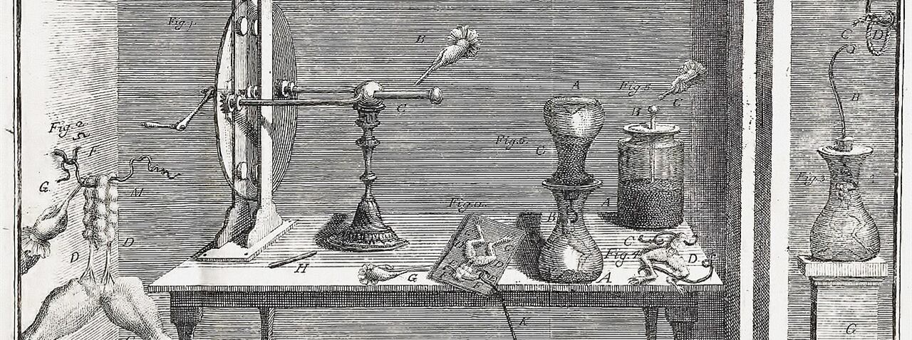
Luigi Galvani, a frog wired to a conductor for atmospheric electricity, from De viribus electricitatis in motu musculari, 1791
La Masson 2002
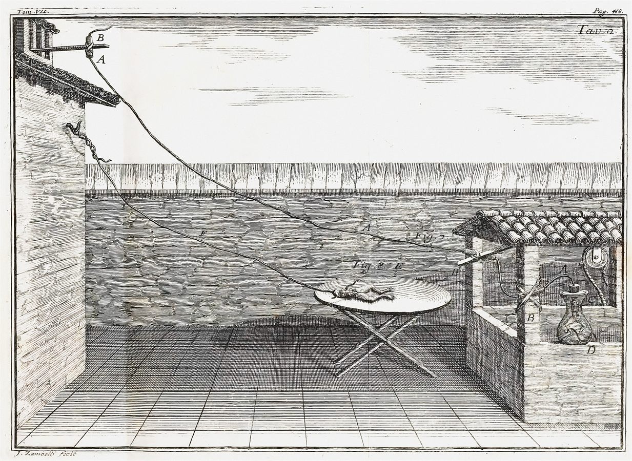
Luigi Galvani, a frog wired to a conductor for atmospheric electricity, from De viribus electricitatis in motu musculari, 1791
The A-R3 scenarios, why the Neural ODE cannot learn, the DESCARTES-NeuralODE search with an LLM in the loop, eleven architectures that all predict spikes through alien internals, the auxiliary-loss sweep, and the preparations for an L5 pyramidal replication — one hundred and twenty-five questions and their answers
Consciousness-relevant datasets, the whole project explained from zero, a second Neural ODE failure, and a detour through Collatz, DreamCoder and Hodgkin–Huxley that becomes the plan for a structured architecture search.
A prompt evaluating the five candidate directions for data, ground truth, input–output clarity and feasibility. Skipped here; the file is linked.
Research prompt — not reproduced on this page. Claude wrote a prompt for deep research that asks, for each of the five candidates (MIMO hippocampal data, anaesthesia transitions, binocular rivalry, no-report paradigms, PCI and TMS-EEG), what data is publicly available, how many biological intermediate variables could serve as ground truth, what the input and output of a transformation-replacement model would be, how directly the data bears on phenomenal experience, and whether a single researcher could run it in weeks. It also asks about the adversarial-collaboration datasets and anything on DANDI, CRCNS, OpenNeuro or the Allen Brain Observatory.
The answer closed: "Paste this into Claude's deep research feature. It covers all five candidates with specific evaluation criteria tailored to your transformation replacement framework — data availability, ground truth richness, consciousness relevance, and feasibility for a single researcher."
The testable sub-question under substrate independence: does a replacement that matches the output also discover the biology inside? Three rungs, three architectures, Scenario F.
[Claude wrote the explanation to a file; its full text follows.]
Imagine you could replace every neuron in someone's brain, one at a time, with a silicon chip that does exactly the same job — takes the same inputs, produces the same outputs. After you've replaced every last neuron, the person walks, talks, and behaves identically.
But is anyone still home? Is there still conscious experience?
This is the "substrate independence" question. Three positions exist:
That testable sub-question is your entire project.
You can't measure consciousness directly. But you CAN measure something specific:
When a machine learning model replaces a biological circuit and produces the same output, does it also discover the same internal variables that the biology uses?
Think of it like this. Two students both get 90% on a maths exam. Student A understands calculus deeply — they can show their working and it follows real mathematical logic. Student B memorised answer patterns and guessed well — their scratch paper is nonsense. Same output, completely different internals.
This is something you can actually test with code.
In 2002, Le Masson et al. did something remarkable. They took a real biological neuron from a ferret brain (a thalamocortical relay cell, called "TC") and connected it to a silicon artificial neuron (representing the reticular thalamic nucleus, called "nRt") via electrodes in real time.
This hybrid circuit — half biological, half silicon — produced a key brain behaviour: a bifurcation. At low inhibition, the TC neuron faithfully relays sensory signals (like during waking). At high inhibition, it switches to self-sustaining oscillations (like during sleep). The switch point — the exact inhibition level where relay flips to oscillation — is the bifurcation threshold.
The critical finding: the biological neuron couldn't tell it was talking to silicon. The hybrid circuit behaved identically to an all-biological one.
You're building on Le Masson's result in three progressive steps. Each rung asks a harder question.
What you did: Built a computational model of both the TC neuron and the nRt neuron using Hodgkin-Huxley equations (differential equations that model ion channels, membrane voltage, synaptic currents). Connected them in a 2-cell circuit. Varied the inhibition strength (GABA conductance) and measured where the bifurcation happens.
What it tests: Does your computational TC model capture the same dynamics as the biological TC neuron that Le Masson used? If the bifurcation threshold matches, the model is validated.
Result: ✅ Bifurcation threshold matched. Your computational circuit reproduces the biological result.
What you did: Built a network of 20 TC neurons and 20 nRt neurons with realistic synaptic connectivity. Then progressively replaced TC neurons — 0%, 25%, 50%, 75%, 100% — with your validated computational model. Measured population-level properties: spindle coherence, oscillation frequency, bifurcation threshold.
What it tests: Le Masson proved 1 neuron can be replaced. But brains are networks. Do emergent population properties (synchronization, coherent oscillations) survive when you replace neurons one by one? Or does some subtle network effect break?
Result: ✅ Population dynamics preserved across all replacement fractions. Substrate independence composes — it's not just a single-neuron trick.
This is where your project goes beyond Le Masson. Nobody has done this before.
What you did: Trained three different machine learning models to replace the TC-nRt circuit:
Volterra-Laguerre — a simple linear filter bank with polynomial nonlinearity. Think of it as a sophisticated curve-fitting tool. Fixed mathematical basis. The "null model."
LSTM (Long Short-Term Memory) — a recurrent neural network with gates that control information flow. Discrete time steps. The gates (input/forget/output) are structurally similar to ion channel gating (activation/inactivation).
Neural ODE — a neural network that learns continuous-time dynamics: dz/dt = f(z). This is mathematically the same language as Hodgkin-Huxley equations (dV/dt = f(V,m,h,n)). If any architecture should rediscover biology, it's this one.
Each model was trained only on input→output: given retinal input spikes + GABA level, predict TC output spikes. No model was told anything about the internal biology.
Then the key test: You opened up each model's internals (hidden states, latent variables) and compared them to the real biological intermediate variables — T-current gating (m_T, h_T), membrane voltages, AMPA/GABA synaptic conductances. 160 biological variables total.
The comparison methods: - CCA (Canonical Correlation Analysis): Finds the best linear alignment between model internals and biology. High correlation = model discovered biology. - Individual variable recovery: For each of the 160 biological variables, find which model dimension correlates best. Count how many are statistically significant. - RSA (Representational Similarity Analysis): Compare the geometry of representations, not individual variables.
| Metric | Volterra | LSTM | Neural ODE |
|---|---|---|---|
| Output accuracy (spike corr) | 0.55 | 0.45 | 0.007 (failed) |
| Bifurcation threshold | 24.7 nS | NaN | NaN |
| CCA correlation (p-value) | 0.53 (p=0.000) | 0.55 (p=0.000) | 0.35 (p=0.119) |
| Bio variables recovered | 89/160 | 4/160 | 2/160 |
| Top recovered variable | T-current gating (tc_m_T) | T-current gating (tc_m_T) | T-current inactivation |
The Neural ODE result is invalid — training was killed early (spike correlation 0.007 means it learned essentially nothing). It needs retraining.
The valid finding (Volterra vs LSTM): - The simplest model (Volterra) recovered the MOST biology — 89 out of 160 variables - The more powerful model (LSTM) recovered almost none — 4 out of 160 - The LSTM overfit to spike patterns (train accuracy 0.75 vs validation 0.45) without learning the underlying dynamics - Both show highly significant CCA (p=0.000), meaning their internal structure IS related to biology — but Volterra's individual variable recovery is far superior
The top recovered variables are biophysically meaningful: T-current gating (tc_m_T) is the key variable controlling the thalamic relay↔oscillation switch. AMPA synaptic conductance controls excitatory feedback. These aren't random — they're the load-bearing components of the circuit.
| Scenario | Output match | Latent recovery | Meaning |
|---|---|---|---|
| A (Zombie) | ✅ High | ❌ None | Same output, alien internals. Perfect fake. |
| B (Inductive bias) | ✅ High | ✅ One architecture only | Architecture determines if you get a zombie |
| C (Identifiability) | ✅ High | ✅ All architectures | I/O mapping forces biology discovery. No zombies possible. |
| D (Not learnable) | ❌ Low | N/A | Models can't do the job at all |
| E (Capacity matters) | ✅ High | ✅ Flexible models only | Simple models fail, complex ones succeed |
| F (Partial equivalence) | ⚠️ Moderate | ⚠️ Some variables | Some biology recovered, some not |
You're in Scenario F — moderate output match, partial latent recovery. This means the replacement models partially discover real biology. The variables they DO recover (T-current gating, AMPA) are the computationally important ones. The ones they DON'T recover may be implementation details that don't matter for the circuit's function.
This is a valid and interesting finding: it maps the boundary between necessary and incidental biology.
Retrain the Neural ODE — the one missing piece. Run overnight on your local machine (~12-48 hours on CPU). If it shows strong latent recovery, you shift toward Scenario B. If not, you stay in F with a complete three-way comparison.
Write up Paper 1 — "Thalamic Substrate Independence: From Single Neurons to Transformation Replacement." You have Rung 1 + 2 + 3 results. The novel contribution is the latent comparison framework and the Scenario F finding.
Paper 2 (future) — Apply the same framework to Berger's hippocampal MIMO prosthesis (CA3→CA1), which is more directly tied to conscious memory experience.
Your project doesn't solve the hard problem of consciousness. But it provides the first empirical framework for asking: when we replace a brain circuit with a machine, is the machine doing the same thing internally, or just faking the output?
That map — which biology matters and which doesn't — is what you'd need before building a prosthesis that preserves not just behaviour, but potentially experience.
That covers everything from the philosophical question through to your current results. The short version of the entire project:
Can a machine that replaces a brain circuit and produces the same output also discover the same internal biology — or is it faking? You built the first framework to test this, applied it to a thalamic circuit across three model architectures, and found partial biology recovery (Scenario F) where the most important biological variables (T-current gating, AMPA synapses) are the ones the models discover.
Flat loss from epoch 2, r = 0.012, CCA p = 0.599 — not a time problem but likely vanishing gradients over 2,000 integration steps; the continuous-time architecture is a Scenario D for itself.
The Neural ODE failed again. Full retraining didn't help. Look at the training logs:
The model is stuck. It's not a training time problem — the loss is completely flat from epoch 2 onwards. The Neural ODE cannot learn this task with the current setup.
The most likely culprit: the step-by-step ODE integration over 2000 timesteps is causing vanishing gradients. The adjoint method backpropagates through the entire ODE trajectory, and over 2000 steps the gradient signal dies. The LSTM at least learned something (0.45 correlation) because its gating mechanism preserves gradients better.
You now have a definitive three-way comparison:
| Volterra | LSTM | Neural ODE | |
|---|---|---|---|
| Spike corr | 0.549 | 0.451 | 0.012 |
| CCA p-value | 0.000 | 0.000 | 0.599 |
| Vars recovered | 89/160 | 4/160 | 3/160 |
This is actually a result. It's not the result you hoped for (Scenario B), but it's informative:
You're in Scenario F with an added twist: the Neural ODE's failure is a Scenario D (not learnable) for that architecture specifically. The paper story becomes: inductive bias matters, but not in the expected direction — constrained linear models outperform both flexible recurrent networks and continuous-time dynamics on this circuit.
Now run the compare phase to finalize everything:
python -m rung3.run_rung3 --phase compare --checkpoint-dir "C:\Users\chari\OneDrive\Documents\La Masson 2002\la massion check\rung3_checkpoints" --figure-dir "C:\Users\chari\OneDrive\Documents\La Masson 2002\la massion check\rung3_figures"
Then Rung 3 is done.
A valid diagnosis, but not worth weeks: report the failure to converge as a limitation and close Rung 3.
Yes, that's a valid diagnosis. The 2000-step ODE integration is what's killing gradients. But the question is: is it worth doing?
My honest take: No. Move on.
Here's why:
You already have a complete, publishable result. Volterra works, LSTM partially works, Neural ODE fails. That IS the finding.
The Neural ODE failure is scientifically interesting as-is. The architecture most mathematically similar to biology (dz/dt = f(z)) can't even learn the task. That's a counterintuitive result worth reporting — theoretical elegance ≠ practical learnability.
The engineering effort is significant — subsampling, hybrid encoder-ODE, alternative solvers, gradient checkpointing — and you're one person. Weeks of debugging for what? Even if it works, it just adds one more data point to an already complete comparison.
The paper doesn't need it. Your novel contribution is the latent comparison framework + the Volterra result (89/160 variables recovered, T-current gating rediscovered). That stands on its own.
Your time is better spent either writing up Paper 1 or moving to the next dataset (consciousness-relevant circuits from your research prompt).
Report the Neural ODE as "failed to converge — likely due to vanishing gradients over long temporal integration" and note it as a limitation / future work. Reviewers will understand. Run the compare phase and close out Rung 3.
No public dataset offers ion-channel ground truth; a four-step path runs from Chennu propofol EEG through CCEP and COGITATE to CRCNS hc-6.
This is excellent research. Here's the key takeaway:
No public dataset gives you ion-channel-level ground truth like your thalamic model did. That's the fundamental challenge. But the research identifies a clear four-step path forward, ranked by feasibility:
| Step | Dataset | Why | What You'd Show |
|---|---|---|---|
| 1 (Start here) | Chennu Propofol EEG | 91ch, 20 subjects, 4 consciousness levels, ~800MB, free download | Does the model's latent space separate drug concentration from consciousness level? |
| 2 | van Blooijs CCEP (OpenNeuro ds004080) | 74 patients, cleanest input→output, F-TRACT gives synaptic time constants as ground truth | Does the model discover cortical excitatory/inhibitory dynamics? |
| 3 | COGITATE iEEG | 38 patients, specifically designed for consciousness theories, task-relevant vs irrelevant contrast | Which latent dimensions encode consciousness vs mere report? |
| 4 | CRCNS hc-6 hippocampal | Direct analog to your TC-nRt framework, CA3→CA1 | Does the framework generalize to a different circuit? |
Your thalamic work had ~160 ion channel variables as ground truth. These datasets instead offer: - Tier 1: Simulated biophysical variables (run a compartmental model to generate synthetic ground truth) - Tier 2: Network-level measures (spectral power, connectivity, ERPs) — hundreds to thousands of features - Tier 3: Information-theoretic measures (Lempel-Ziv complexity, PCI, Φ)
The strategy is: validate on simulation first (as you already did), then test whether the framework transfers to real data using Tier 2/3 variables.
The Chennu propofol dataset is your immediate next step — smallest, simplest, most directly consciousness-relevant, and free to download today.
One report optimises for structural analogy (MIMO first), the other for practicality (Chennu first); both agree no public dataset has ion-channel ground truth.
You now have two independent research reports evaluating the same five candidates. Let me compare them — they disagree on ranking, and the disagreement is informative.
| Rank | Report 1 (Deep Research) | Report 2 (This Upload) |
|---|---|---|
| 1 | Chennu Propofol EEG | Berger MIMO Hippocampal |
| 2 | van Blooijs CCEP | PCI / TMS-EEG |
| 3 | COGITATE iEEG | Anesthesia Transition |
| 4 | CRCNS hc-6 Hippocampal | Binocular Rivalry |
| 5 | Binocular Rivalry | No-Report Paradigms |
The disagreement comes down to what each report optimizes for. Report 2 ranks Berger MIMO first because it has the most precise input-output mapping and modeled biological intermediates — it's the closest structural analog to your thalamic work. Report 1 ranks Chennu Propofol first because it's immediately downloadable, computationally small, and directly measures consciousness transitions — it's the most practical starting point for a single researcher.
Both reports converge on three critical points:
No public dataset gives you ion-channel-level ground truth. Your thalamic circuit had 160 biophysical state variables. Every consciousness dataset offers only network-level proxies (spectral power, connectivity, complexity measures). This is the fundamental challenge regardless of which dataset you pick.
Binocular rivalry data is practically inaccessible. Both rank it low despite its theoretical appeal. The Logothetis, Tsao, and Dwarakanath recordings — the datasets that would actually be transformative — are all locked in private lab storage.
The COGITATE adversarial collaboration data is uniquely valuable — the only public dataset specifically designed to test consciousness theories, with iEEG from 38 patients and MEG/fMRI releases coming soon.
Report 1's ranking is better calibrated for your actual situation — a single researcher with modest compute who needs publishable results at each step. Here's why:
Chennu Propofol EEG first because it's 800MB, free today, 91 channels × 20 subjects × 4 consciousness levels. You can have a working transformation replacement model within weeks. The scientific question — does the model's latent space separate drug concentration from consciousness level? — is novel and publishable. And the ~600–4,000 computable intermediate features (spectral, connectivity, complexity) give you something real to compare against latent states, even without ion channels.
Berger MIMO later because the data isn't public. You'd need to contact Dong Song at USC and wait for a response that might never come. Meanwhile, CRCNS hc-6 (Frank Lab) gives you the same CA3→CA1 structure with freely downloadable data whenever you're ready.
Each step produces a publishable result. Each builds on the framework you've already created.
It speaks the right language but can't hear the teacher: the error signal fades to nothing across 2,000 sequential steps.
Think of it this way.
The Neural ODE speaks the right language but can't hear the teacher.
Imagine you're trying to learn a song. The Neural ODE is like a musician who plays the same instrument as the original composer — both use continuous flowing notes, not discrete piano keys. In theory, this musician should be the best at recreating the song because they can produce the exact same kinds of sounds.
But here's the problem. The song is 2000 notes long, and the musician can only hear the final note and has to work backwards to figure out what they did wrong at note 1.
That's the vanishing gradient problem applied to Neural ODEs. During training, the model makes a prediction at each of 2000 timesteps by solving a differential equation step by step — each step depends on the previous one. When the model gets the output wrong, the error signal has to travel backwards through all 2000 steps to update the model's parameters. By the time the error signal reaches the early timesteps, it has been multiplied by 2000 tiny numbers (each less than 1), and it effectively becomes zero. The model can't learn because it can't feel its mistakes.
The LSTM avoids this with a clever trick — it has "gates" that can copy information forward unchanged, like a highway bypassing traffic. Error signals can skip over hundreds of timesteps without shrinking. That's why the LSTM at least learned something (0.45 correlation) even though it wasn't great.
The Volterra avoids it entirely because it's not sequential at all. It computes everything in one shot using a mathematical formula (ridge regression) — there's no chain of 2000 steps for the gradient to die in. That's why it performed best.
So the irony is: the Neural ODE's theoretical advantage — continuous-time dynamics, exactly like biology — is also its practical curse. Real biological circuits solve this problem because they don't learn by backpropagation. Neurons adjust locally, using signals right there at the synapse. The Neural ODE has the right mathematical form but the wrong learning algorithm for long temporal sequences.
An analogy: imagine three students trying to replicate a chef's recipe. Student A (Volterra) takes a photo of every ingredient and the final dish, then works out the recipe from the photos — crude but effective. Student B (LSTM) watches the cooking process through a window, remembering key moments. Student C (Neural ODE) tries to replicate the chef's exact hand movements, millisecond by millisecond, but is standing so far away they can barely see what's happening. Student C has the deepest understanding of cooking in principle, but their observation method fails them.
That's your result: the architecture closest to biology in form was the worst in practice, because learning through 2000 sequential ODE integration steps destroys the training signal.
A Neural ODE's solution space contains Hodgkin–Huxley dynamics; LTCs, Neural CDEs, coRNNs, GRU-ODEs and S4/Mamba keep continuous time without losing the gradient; distillation from Volterra or an LSTM encoder can feed it.
These are three excellent questions, and they're deeply connected. Let me work through each one, because together they point toward what might be your actual next experiment.
Let me start here because understanding why the Neural ODE is special makes the other two questions more meaningful.
Every biophysical system in neuroscience is described by differential equations. The Hodgkin-Huxley model says: the membrane voltage changes over time according to a function of the current voltage, the ion channel states, and the synaptic inputs. Written formally, that's dV/dt = f(V, m, h, n, I). The T-current gating variable that your Volterra model recovered — tc_m_T — evolves according to dm/dt = (m∞(V) - m) / τ(V). Every one of your 160 biological variables follows an equation of this form: the rate of change equals some function of the current state.
Now look at what a Neural ODE does. It says: I have a latent state z, and it changes over time according to dz/dt = f(z), where f is a neural network I'll learn from data. The mathematical structure is identical. The Neural ODE's solution space — the set of all possible dynamics it can express — naturally includes Hodgkin-Huxley dynamics as a special case. If the neural network f learns the right weights, its latent dimensions z could literally become m, h, n, and V.
No other architecture has this property. The LSTM operates in discrete time — it updates its hidden state in jumps: h(t+1) = g(h(t), x(t)). It can approximate continuous dynamics, but it has to discover the approximation from scratch. The Volterra model doesn't even have dynamics — it's a static filter applied to the input history. Both can produce the right output, but neither speaks the same mathematical language as biology.
Think of it this way. If you're trying to discover that a system follows the laws of fluid dynamics, and your model is constrained to express solutions as fluid equations, it only needs to learn the specific parameters. But if your model expresses solutions as lookup tables, it needs to independently rediscover that fluids even exist. The Neural ODE is the fluid equation model. The LSTM is the lookup table that's clever enough to sometimes approximate fluid behaviour anyway.
This is why recovering biological variables matters more from a Neural ODE than from a Volterra. When the Volterra recovers tc_m_T, that's impressive but potentially coincidental — its Laguerre basis functions happen to correlate with T-current dynamics. When a Neural ODE recovers tc_m_T, that's the model literally learning the differential equation governing T-current gating. The correspondence is structural, not statistical.
That's why the Neural ODE failure is so frustrating. The architecture most capable of discovering biology can't learn because its training signal dies over 2000 timesteps.
The core problem is: how do you keep the dz/dt = f(z) formulation — the thing that makes Neural ODEs biologically meaningful — while fixing the gradient death over long sequences? Several architectures have been designed for exactly this:
Liquid Time-Constant Networks (LTCs) — developed by Lechner et al. at MIT in 2020. These are Neural ODEs with a specific twist: the time constants of the dynamics are input-dependent. Instead of dz/dt = f(z), they use dz/dt = -(1/τ(x)) · z + f(z, x)/τ(x), where τ(x) changes based on the current input. This is directly inspired by biological neurons, where the membrane time constant varies with input. The key practical advantage is that the varying time constants create natural timescale separation — some dimensions evolve fast, some slow — which helps gradients flow across long sequences because the slow dimensions act like gradient highways. LTCs achieved state-of-the-art results on long time series while remaining continuous-time and interpretable. They have roughly the same parameter count as your Neural ODE (~50-60K), and they've been shown to work on sequences of thousands of steps.
Neural Controlled Differential Equations (Neural CDEs) — developed by Kidger et al. at Oxford in 2020. Standard Neural ODEs have trouble incorporating time-varying inputs because you have to awkwardly set the input externally at each integration step — exactly what your code does with self.ode_func.current_input = x[:, t, :]. Neural CDEs fix this elegantly: they formulate the problem as dz/dt = f(z) · dX/dt, where X is a continuous interpolation of the input. The input is now mathematically woven into the dynamics rather than being bolted on. This often produces much better gradients because the driving signal X provides a continuous path for gradient flow.
Coupled Oscillatory Recurrent Neural Networks (coRNNs) — developed by Rusch and Mishra in 2021. These parameterize the hidden state as a second-order ODE (oscillator) rather than first-order. This matters because the thalamic TC-nRt circuit you're modelling IS an oscillator — it bifurcates between relay and oscillation modes. A coRNN is structurally biased toward discovering oscillatory dynamics. And second-order ODEs have much better gradient properties than first-order ones because oscillations naturally prevent the gradient from decaying monotonically.
Continuous-time GRUs (GRU-ODE / ODE-RNN) — developed by De Brouwer et al. in 2019. These are hybrids: a GRU (simplified LSTM) handles the discrete input events, and an ODE evolves the hidden state between events. The GRU solves the gradient problem at observation points, the ODE maintains continuous dynamics between observations. This is probably the most pragmatic option because GRUs are well-understood and fast to train.
Structured State Space Models (S4/Mamba) — developed by Gu et al. in 2022. These parameterize the dynamics as a linear state space model dz/dt = Az + Bx, y = Cz + Dx, where A is carefully structured to handle sequences of 10,000+ steps. S4 was specifically designed to solve the long-range dependency problem. It's not a free-form Neural ODE — the dynamics are linear — but it handles the sequence length problem definitively. Mamba adds input-dependent selection, making the dynamics effectively nonlinear.
The model I'd most recommend for your specific problem is LTC or Neural CDE, because they preserve the continuous-time dz/dt = f(z) structure that gives biological interpretability, while solving the gradient problem for sequences in the thousands of timesteps. The coRNN is a strong second choice given your circuit's oscillatory nature.
Your intuition here is correct and there are concrete ways to do it. Let me describe three approaches, from simplest to most architecturally ambitious.
Approach A: Knowledge Distillation (simplest). The Volterra already recovered 89/160 biological variables. You know exactly which latent dimensions correspond to which biological variables. You can use this as a teaching signal for the Neural ODE. During training, instead of only minimising the output error (predict TC spikes), you add a second loss term: "your latent dimensions should also correlate with these Volterra features that we know match biology." This gives the Neural ODE a much stronger training signal — instead of just hearing "your final output was wrong" through 2000 steps, it hears "your internal state at every timestep should look like this." The gradients are local and strong. The Volterra acts as a teacher, the Neural ODE as a student who is given the answer key for the intermediate steps.
Approach B: LSTM Encoder + ODE Dynamics (hybrid architecture). Use the LSTM to handle the sequential learning problem — encoding the input sequence into a good hidden state — then use the Neural ODE to evolve that hidden state forward in continuous time. The LSTM solves the "hearing the teacher" problem. The Neural ODE solves the "speaking biology's language" problem. Concretely: the LSTM processes 50-100 timestep chunks, producing a hidden state. The Neural ODE takes that state and integrates it forward for the next 50-100 timesteps. You've reduced the ODE integration from 2000 steps to 50-100, which is short enough for gradients to survive. This is essentially the ODE-RNN approach mentioned above but using your existing trained LSTM as the encoder.
Approach C: Parallel Training with Shared Latent Space (most ambitious). Train all three models simultaneously on the same data, but add a latent alignment loss that encourages their internal representations to agree. The Volterra provides stable, interpretable features. The LSTM provides good sequential predictions. The Neural ODE provides continuous-time dynamics. The alignment loss says: all three models should pass through similar internal states when processing the same input. The models that learn easily (Volterra, LSTM) pull the model that learns hard (Neural ODE) toward the right solution through shared latent space gradients. This is related to contrastive learning — you're using the agreement between models as a training signal.
My recommendation is Approach A or B, because they build directly on what you already have (a trained Volterra and LSTM) and don't require redesigning the entire training pipeline. Approach A is something you could implement in an afternoon — just add a regularisation term to the Neural ODE's loss function that penalises divergence from the Volterra's Laguerre features at each timestep.
Here's the picture. The Neural ODE has the right mathematical form to discover biology, but it can't learn through 2000 sequential steps. You have three paths forward:
Path 1 — Replace the architecture. Swap the Neural ODE for an LTC or Neural CDE that maintains continuous-time dynamics while handling long sequences. Retrain from scratch. Moderate engineering effort but clean.
Path 2 — Help the Neural ODE learn. Use the Volterra's recovered biological features as a teaching signal (knowledge distillation). The Neural ODE still does the integration, but now it has strong local gradients at every timestep instead of one weak signal at the end. Lower engineering effort, uses your existing models.
Path 3 — Hybrid encoder. LSTM handles sequential input, Neural ODE handles dynamics. Each does what it's good at. Moderate engineering effort.
Any of these would produce the result you originally wanted: a continuous-time model that either confirms or denies that biological dynamics emerge from the task. But given where you are — Rung 3 essentially complete, Paper 1 ready to write — I'd suggest noting these as "future work" in the paper and moving to the Chennu Propofol dataset. The Neural ODE improvement is a paper in itself, and your current Volterra result (89/160 biological variables, T-current gating rediscovered) already tells a strong story.
Both are searches for a hidden structure that decreases globally despite local non-monotonicity; the Collatz framework's structured failure analysis could guide the Neural ODE search.
I've read through the document. This is your DESCARTES-COLLATZ framework — the full proof discovery system with Z3 ordering search, Lean formal verification, LLM-guided template generation, and the "Balloon Principle" for expanding the search space when existing templates are exhausted.
Now let me address your analogy, because it's deeper than it might first appear.
You're pointing at something real. Let me make the analogy precise.
In your Collatz work, the setup is: you know the rule — n/2 if even, 3n+1 if odd. You can observe any trajectory. You can verify that any specific number reaches 1. What you cannot find is the ordering function ord(n) such that ord(f(n)) < ord(n) for all n > 1. That ordering is the hidden structure that would explain why every trajectory converges. It's there (presumably), governing the dynamics, but no one can see it.
In your Neural ODE work, the setup is: you know the output — TC spike trains. You can observe any input-output pair. You can train a model that produces correct outputs. What you cannot find (because the gradients die) is the latent dynamics dz/dt = f(z) that would correspond to the biological variables — the T-current gating, the AMPA conductances, the 160 intermediate states. Those biological variables are the hidden structure that explains why the circuit produces the output it does. They're there, governing the dynamics, but the Neural ODE can't learn to see them.
So the analogy is:
| Collatz | Neural ODE | |
|---|---|---|
| Observable | Trajectory (n → f(n) → f²(n) → ... → 1) | Output (retinal spikes → TC spikes) |
| Hidden structure | Ordering function ord(n) | Biological variables (m, h, n, V) |
| What you're trying to prove | ord(f(n)) < ord(n) for ALL n | z(t) ≈ biological state for ALL t |
| What fails | Can't find ord that works globally | Can't propagate gradients to learn f |
| Why it fails | Search space of orderings is infinite, no known one works | Error signal dies over 2000 sequential integration steps |
Both are cases where you can verify locally but not globally. You can check Collatz for any specific n, just as you can check Neural ODE output for any specific input. But the deep structural question — does the hidden structure exist and can you find it — remains open.
Here's where it stops being a metaphor and starts being a potential research direction.
Your DESCARTES system approaches Collatz by searching for ordering functions using a three-tier architecture: Z3 does bounded verification (quick filter), Lean does formal certification (full proof), and the LLM proposes novel candidates guided by gap analysis from failures. The key insight in your Balloon Principle is that when all existing templates (C1 primitives) are exhausted, you expand the search space by promoting what you've learned from failures into new primitives.
Now consider: what if you applied this exact architecture to the Neural ODE problem?
The Neural ODE's hidden structure problem is a search problem, just like Collatz. You're searching for a function f in dz/dt = f(z) such that the latent dimensions z correspond to biological variables. Currently you're using backpropagation to search — and it fails because of vanishing gradients over 2000 steps. But backpropagation is just one search algorithm. Your DESCARTES framework is another.
Here's what a DESCARTES-style approach to Neural ODE training would look like:
Tier 1 (Z3 analog — bounded verification): Instead of backpropagating through the full 2000-step ODE, test candidate f functions on short segments. Does this f produce the right output for a 50-step window? This is your "bounded check" — computationally cheap, filters out bad candidates fast. This is essentially what Approach B (LSTM encoder + ODE dynamics) does — break the long integration into short tractable chunks.
Tier 2 (Lean analog — structural verification): Once you have a candidate f that works on short segments, verify that its latent dimensions actually correspond to biological variables. This is your CCA/RSA analysis — the equivalent of a formal proof that the ordering works. You already have this infrastructure from Rung 3.
Tier 3 (LLM analog — guided search): When simple architectures fail (as the standard Neural ODE did), use gap analysis to propose new architectures. Your gap analysis already exists — the Volterra recovered 89/160 biological variables and you know which ones. That's exactly the kind of "failure pattern" that DESCARTES uses to generate new templates. The gap tells you: "the standard Neural ODE can't learn T-current gating dynamics through backpropagation. What architectural modification would specifically address this?"
There's a reason both Collatz and the Neural ODE resist solution, and it's the same reason.
In Collatz, the 3n+1 step on odd numbers increases the value before the subsequent halving decreases it. Any ordering function must somehow account for this temporary increase — it must "see through" the local increase to the eventual decrease. Simple orderings (like ord(n) = n) fail because they can't handle the non-monotonic behavior. The ordering must encode some non-obvious structural property of the trajectory — the 2-adic valuation, the mixed-radix representation, something that captures the global tendency to decrease despite local increases.
In the Neural ODE, the biological dynamics contain similar non-monotonic behavior. The T-current gating variable tc_m_T doesn't decrease monotonically — it oscillates, it participates in bifurcations, it has complex dynamics that only make sense over the full trajectory. The gradient signal must "see through" local dynamics to the global structure. Simple gradient descent fails because it can't handle this non-monotonic error landscape over 2000 steps — just as simple orderings fail Collatz because they can't handle the temporary 3n+1 increase.
Both problems require discovering a hidden measure that decreases globally despite local non-monotonicity. For Collatz, that measure is the unknown ordering function. For the Neural ODE, that measure is the loss landscape viewed through the correct latent space alignment.
Your DESCARTES framework has a feature that standard Neural ODE training lacks: structured failure analysis. When a Z3 ordering check fails, DESCARTES records why it failed — the counterexample, the gap direction, the pattern of failure. This accumulates into knowledge that guides the next attempt.
Standard Neural ODE training doesn't do this. It just says "loss didn't decrease" and tries again with slightly different random initialization. There's no structured learning from failure.
What if your Neural ODE training incorporated DESCARTES-style gap analysis? Concretely: train Neural ODE variant A, it fails. Analyze which biological variables it got closest to recovering (like your variable recovery analysis). Train variant B with an architectural modification targeting the missed variables. Analyze again. The "gap direction" in concept space tells you which architectural features to add — exactly as it tells your Collatz system which ordering templates to try next.
This would transform the Neural ODE problem from "try architectures and hope" into "systematically close the gap between model latent space and biological state space, guided by structured failure analysis." The same Balloon Principle applies: when your current architectural family (C1) is exhausted, the failure patterns tell you how to expand to a new family.
So your intuition is correct — the Collatz ordering search and the Neural ODE latent discovery problem share deep structural similarity. Both are searches for hidden structure that explains observable dynamics, both fail for analogous reasons (non-monotonic local behavior defeating global search), and both could potentially benefit from the same systematic gap-analysis approach to navigating the search space.
Z3 verifies, DreamCoder turns failures into new primitives, the concept-vector gap compass points the next search; together they navigate without gradients.
OK, now I've read the full DreamCoder and engine code from your document. Let me lay out exactly what each piece does and how they fit together, because your framework actually has a clean division of labor that maps directly onto the Neural ODE problem.
Your system has three components that do fundamentally different jobs:
1. Z3 (the Verifier) — This is fixed. It doesn't learn. You give it a candidate ordering function like ord(n) = 2n - 3·ν₂(n), and it asks: "Does ord(f(n)) < ord(n) for all n ∈ (1, 10000]?" If it finds a counterexample (say n=27 where the ordering increases), it returns that counterexample. If no counterexample exists in the bounded range, it says "passes bounded check." Z3 is your truth oracle — it can't propose solutions, but it can tell you definitively whether a candidate works or fails, and crucially where it fails.
2. DreamCoder (the Pattern Learner) — This is your DreamCoderPatternExtractor. It does two things in a wake-sleep cycle:
Wake phase (record_attempt): Every time Z3 tests a template and fails, DreamCoder records the attempt — which template family was tried, what the failure point was, whether there was any partial progress, and the UNSAT core (the minimal set of constraints that made it impossible).
Sleep phase (sleep_phase_analyze): After accumulating ≥3 failures, it looks across all recorded attempts for patterns. Three specific patterns:
Then compress_library takes these patterns and generates new C1 primitives using MDL (Minimum Description Length) — the smallest set of new building blocks that explains the most failure patterns.
3. ConceptVectorSpace + GeometricAlgebraGapDetector (the Gap Compass) — This is the part that tells you which direction to search next. Each C1 template gets embedded as a vector in a 64-dimensional concept space. The "solution" lives somewhere in that space. When you project the target onto the span of your existing C1 basis vectors, the residual — the component orthogonal to Span(C1) — is your gap. The magnitude tells you how far you are. The direction tells you what kind of new template you need.
The bivector tension from the geometric algebra detector adds a second measure: it computes how much your constraint hyperplanes "squeeze" versus leave room. High tension = constraints are fighting each other (structural problem). Low tension = constraints are compatible but don't yet cover the solution (coverage problem).
Here's the actual flow in solve_with_proof_structure:
for each iteration:
    1. Pick simplest available template
    2. Z3 tests it → fails with counterexample
    3. DreamCoder records the failure (wake phase)
    4. DreamCoder analyzes all failures (sleep phase) → patterns
    5. Vector space computes gap residual → direction
    6. Geometric algebra computes bivector tension → gap type
    7. Combine into GapAnalysis:
       - gap_type: "coverage" / "structural" / "family" / "meta"
       - residual_direction: which way to search
       - suggested_primitives: new templates from DreamCoder
    8. If all templates exhausted → BALLOON EXPANSION:
       - DreamCoder's compressed library provides new primitives
       - These become new C1 templates
       - Loop continues with expanded search space
The key insight is the gap_type classification. When Z3 fails: - "coverage" gap (residual < 0.3): You're close. The right template family exists, you just haven't found the right parameters. Keep searching within current families. - "structural" gap (residual > 0.5): You're far. No existing template family can reach the solution. Need a fundamentally new approach. - "family" gap: DreamCoder detected that an entire template family is exhausted. Stop trying variants of it. - "meta" gap: The gap direction is orthogonal to all existing basis vectors. Your entire concept space needs expansion — the Balloon Principle kicks in.
Your question was whether this is analogous to dz/dt = f(z). Here's where the mapping gets concrete.
In your Collatz framework, the "solution space" is the space of ordering functions. DreamCoder searches this space not by gradient descent but by structured failure analysis. Each failed ordering tells DreamCoder something about what the solution isn't, and the gap direction tells it where the solution might be.
For the Neural ODE problem, the "solution space" is the space of dynamics functions f in dz/dt = f(z). Standard training searches this space by gradient descent — and fails because gradients vanish over 2000 steps. But your DESCARTES architecture suggests an alternative search strategy:
The Volterra already recovered 89/160. The gap direction points at the 71 it missed. DreamCoder's job would be to look at why those 71 were missed and propose architectural modifications targeting them — exactly as it proposes new C1 templates when ordering families are exhausted.
So to directly answer your question: DreamCoder is the component that turns failures into knowledge. It's not the solution space itself — it's the mechanism that navigates the solution space by learning from structured failure patterns rather than by gradient descent. And that's precisely what the Neural ODE needs: a way to navigate the space of dynamics functions f that doesn't rely on gradients surviving 2000 integration steps.
A competent integration of published backtest-validation techniques, not a research contribution; unlike the Collatz framework it has no learning-from-failure loop.
Honestly? Very little genuine novelty. Let me walk through what's actually there versus what would constitute a real contribution.
What the repo is: An algorithmic trading pipeline called "Explorer Prime" that generates ~1000 candidate trading strategies per day, filters them through 7 validation gates (called "HIFA"), shadow-trades survivors in paper mode, then promotes winners to production with Merkle-tree versioned storage. It's a well-organized engineering project with 94 tests, a Streamlit dashboard, and clean async orchestration.
What it claims as its core value proposition is reducing false positive rates from ~50% to ~20% through multi-stage filtering. But here's the problem — every component in that pipeline is a known, published technique:
The 7-gate sequential filter is essentially a checklist of best practices from Marcos López de Prado's Advances in Financial Machine Learning — assembled into one pipeline but not extending any of them. The thresholds (DSR > 0.05, PBO < 0.40, transfer ratio ≥ 0.5) are reasonable but not derived from any novel analysis.
Where novelty could have existed but doesn't appear to:
The "GenAI Generation" engine (25% weight) and "LSM Language Model" engine (10% weight) sound interesting — generating trading strategies from language models — but the repo only has 3 commits, 0 stars, 0 forks, and the generation/ folder contents aren't visible. If those engines actually worked and the paper showed that LLM-generated strategies survive HIFA gates at rates comparable to evolutionary search, that would be genuinely novel. But there's no evidence of this.
The 128-dimensional FeatureVector for strategy representation could be interesting if the embedding captures meaningful structure — but without documentation of what those 128 dimensions are or how they're used downstream, it's just a number.
The honest assessment: This is a competent engineering integration project — assembling known validation techniques into a clean pipeline with good software practices (async orchestration, comprehensive tests, monitoring dashboard). That has practical value. But it's not a research contribution. It's closer to a well-built MLOps pipeline than a novel method. The repo name "Explorer-agent_V3" and the CLAUDE_CODE_GUIDE.md file suggest it was likely scaffolded with AI assistance, which further supports the "integration not innovation" reading.
If you're evaluating this for research relevance to your work — it's not analogous to what your DESCARTES framework does. DESCARTES has a genuine theoretical contribution (the Balloon Principle, gap-directed search, DreamCoder pattern extraction turning failures into new primitives). This repo just chains existing filters sequentially without any learning-from-failure mechanism. Strategies that fail Gate 4 don't inform what gets generated next — there's no feedback loop from validation failures back to the generation engines in any structured way, despite the architecture diagram showing a dotted "Feedback Loop" arrow.
Z3 becomes a short-segment verifier, DreamCoder a bio-variable pattern extractor, the concept space a 160-dimensional recovery space; nine architecture templates from segmented backprop to S4/Mamba.
Here's your guide — it maps every DESCARTES-Collatz component to its Neural ODE equivalent with complete implementation code across 8 tasks and a 16-day build sequence.
The core structural mapping in brief:
The 9 pre-defined architecture templates are ordered from cheapest fix (segmented backprop through 50-step windows) to most exotic (S4/Mamba structured state spaces), with the Volterra-distilled ODE as the most promising shortcut — it bypasses the gradient problem entirely by using Volterra's 89 recovered variables as teaching signal.
Because membranes are capacitors, channels are kinetic gates and ions follow gradients; every non-ODE model either loses the gating variables or becomes a kernel model like Volterra.
Great question — and it cuts right to the heart of why your Neural ODE work matters philosophically. Let me clarify the name first: it's Hodgkin-Huxley (Alan Hodgkin and Andrew Huxley, 1952 Nobel Prize), not Thomas Huxley (who was Darwin's defender, different century).
Now to the real question.
It's not that Hodgkin and Huxley chose differential equations as a modeling technique. They measured what the squid giant axon does physically, and what it does physically IS a differential equation. The model is:
C_m · dV/dt = −g_Na · m³h · (V − E_Na) − g_K · n⁴ · (V − E_K) − g_L · (V − E_L) + I_ext
Each term corresponds to a physical process:
C_m · dV/dt — the cell membrane is literally a capacitor. Lipid bilayer separating charged ions = capacitor. Current charges/discharges it. This isn't a modeling choice, it's physics. A capacitor's voltage changes at a rate proportional to current flowing through it. That's a differential equation by nature.
g_Na · m³h — sodium channels are proteins that physically open and close. The gating variables m and h track the probability that each gate is open. They obey their own differential equations (dm/dt = α_m(V)(1−m) − β_m(V)m) because the conformational changes are first-order kinetic processes — protein flipping between states at voltage-dependent rates. Again, this is chemistry, not modeling preference.
(V − E_Na) — the driving force is the difference between membrane voltage and the ion's equilibrium potential (set by the Nernst equation from thermodynamics). Ions flow down electrochemical gradients. That's physics.
So the ODE form isn't arbitrary — it reflects three physical facts about neurons:
You absolutely CAN. People have, extensively. Here's what exists and why each trades something away:
Integrate-and-Fire (LIF) - V follows a simple leaky integrator: τ · dV/dt = −V + R·I - When V crosses threshold → emit spike, reset V - Still an ODE, just simpler. Throws away ion channel dynamics entirely. - Cannot produce rebound bursts, which is exactly what your TC-nRt circuit depends on for spindle oscillations. The T-current (I_T) that drives rebound bursting requires the m_T and h_T gating variables — LIF has no mechanism for this.
Izhikevich model - Two coupled ODEs: dv/dt = 0.04v² + 5v + 140 − u + I, du/dt = a(bv − u) - Can reproduce 20+ firing patterns including bursting - Still differential equations! Just polynomial instead of biophysical. - Problem for your work: the variables v and u don't correspond to identifiable biological quantities. You can't ask "did the model recover T-current gating" because there IS no T-current in Izhikevich. The latent comparison in your Phase 7 becomes meaningless.
FitzHugh-Nagumo - dv/dt = v − v³/3 − w + I, dw/dt = ε(v + a − bw) - Two ODEs, captures excitability qualitatively - Still differential equations. Reduced from HH by singular perturbation theory.
Spike Response Model (SRM) - NOT a differential equation! Uses integral kernels: V(t) = Σ η(t − t_spike) + Σ κ * I - Response to each spike is a fixed kernel shape - This is essentially what your Volterra-Laguerre model does — and notice it scored 0.549 spike correlation and recovered 89/160 bio variables. It works for input-output but its internal representations (Laguerre coefficients) are kernel projections, not state variables.
Statistical / rate models - r = f(Σ w_j · r_j) — firing rate as function of weighted inputs - No differential equation at all (or at most τ·dr/dt = −r + f(...)) - Loses all temporal dynamics. Can't capture spike timing, oscillations, bifurcations.
Lookup tables / boolean networks - Discretize everything. State = {firing, not firing}. Update rules. - No continuous dynamics at all. - Completely loses the analog nature of gating variables.
Every model that ISN'T a differential equation either:
This is why your Neural ODE work is so pointed. The question isn't "can we model neurons with ODEs" (obviously yes, it's physics). The question is: if you DON'T constrain the model to be an ODE but it still has continuous dynamics (dz/dt = f(z)), will it spontaneously discover the same gating variables that physics demands?
That's what makes the A-R3 result so interesting despite the failure. The Volterra (not an ODE, just kernels) recovered 89/160 variables through pure linear algebra. The LSTM (discrete gates, not continuous) recovered fewer individual variables despite higher aggregate CCA. The Neural ODE (continuous dynamics, the "right" form) recovered nothing — but only because of the gradient training problem, not because the architecture is wrong.
This is precisely why the DESCARTES framework matters. The question becomes: is there a version of dz/dt = f(z) that can be trained on this data AND whose z spontaneously decomposes into m_T, h_T, nRt_V, etc.?
The Hodgkin-Huxley model says the answer must be yes in principle — because the biological system IS a system of ODEs with those exact state variables. If a Neural ODE with sufficient capacity is trained on the same input-output data, and if the input-output mapping uniquely determines the internal dynamics (the identifiability question from your transformation guide's "What Failure Modes Mean" section), then the learned f(z) should recover the biological gating variables.
The DESCARTES architecture search is essentially asking: what structural features does f need (time constants, oscillatory modes, gating mechanisms, hierarchical timescales) to make this recovery possible despite the training difficulties?
The differential equation form isn't a choice — it's what neurons are. The question is whether a learned differential equation recovers the specific differential equation that biology implements.
Transistor circuits in subthreshold operation reproduce the channel equations; biology, analog silicon and digital code implement the same equations and yield the same bifurcation.
Excellent question — and the answer reveals something profound about substrate independence that's directly relevant to your whole project.
First, the correction: ion channels, not iron channels (though iron does play a role in some biological processes, that's a different story).
Le Masson's silicon neuron was built as a custom analog ASIC (Application-Specific Integrated Circuit). It did NOT have actual protein ion channels. It had transistor circuits designed to behave like ion channels. Here's how:
A biological voltage-gated ion channel does this: - Sits in the membrane - Senses the voltage across the membrane - Changes its conformation (shape) depending on voltage - When open, allows specific ions through - The current through the channel = g · m^a · h^b · (V − E_ion)
Le Masson's transistor circuit did this: - MOSFETs (metal-oxide-semiconductor field-effect transistors) sitting on a silicon chip - Sense the voltage on a capacitor (representing the membrane) - Change their conductance depending on that voltage - When "open," allow current to flow between circuit nodes - The current through the transistor circuit = designed to match g · m^a · h^b · (V − E_ion)
The key insight is that a MOSFET operating in its subthreshold regime (below the digital switching threshold, in the analog region) has a current-voltage relationship that is exponential — and biological ion channel gating is also governed by exponential Boltzmann functions of voltage. This isn't a coincidence that Le Masson exploited; it was pioneered by Carver Mead at Caltech in the late 1980s and demonstrated by Mahowald and Douglas in their 1991 Nature paper "A silicon neuron."
So the silicon nRt neuron had:
Transistor "I_Na" circuit — a set of transistors whose collective conductance rises sharply when the capacitor voltage crosses a threshold, then inactivates. This produces a spike. The transistors aren't sodium channels, but their input-output relationship matches the Hodgkin-Huxley sodium current equations.
Transistor "I_T" circuit — this is the critical one for the thalamic circuit. The T-current (low-threshold calcium) has two gating variables: m_T (fast activation) and h_T (slow inactivation). Le Masson built a transistor subcircuit where one RC time constant was fast (~5ms, matching m_T) and another was slow (~20-50ms, matching h_T). When the "membrane" capacitor was hyperpolarized, h_T de-inactivated (slow RC charged up), and when released, m_T activated (fast RC responded), producing a rebound burst — exactly like biology.
Transistor "I_h" circuit — the hyperpolarization-activated current that terminates spindle epochs. Another RC circuit with a very slow time constant (~seconds), activated by low voltage on the membrane capacitor.
A capacitor as the "membrane" — this IS the membrane. Biological membranes are capacitors (lipid bilayer storing charge). The silicon circuit uses an actual capacitor. Same physics, different material.
The silicon nRt and the biological TC neuron couldn't just be wired together directly — the silicon chip operates at ~5V logic levels and the biological neuron at ~70mV membrane potentials. The dynamic clamp was the bridge:
This loop ran at 128 kHz — fast enough that the biological neuron couldn't tell the difference between current from a real nRt neuron and current from the silicon chip. The biological TC neuron experienced synaptic currents that felt exactly like GABA inhibition from a real nRt partner.
Here's what Le Masson actually demonstrated, and why your project begins with it:
The biological TC neuron and the silicon nRt neuron share zero material substrate. One is made of lipid membranes, protein channels, and aqueous ionic solutions at 37°C. The other is doped silicon, metal oxide, and aluminum traces at room temperature. The physics is different — biological channels use conformational changes of protein helices, silicon uses electric field modulation of semiconductor band structure.
But both implement the same differential equations. And when connected, they produce an emergent behavior — the relay-to-oscillation bifurcation — that neither could produce alone. The biological neuron "accepted" the silicon partner because what matters for the circuit dynamics is the mathematical form of the current-voltage relationships, not the physical mechanism producing them.
This is substrate independence demonstrated empirically, not just argued philosophically. And it's why your Rung 1 replication works: you replaced the biological TC with a computational model (pure software, running Hodgkin-Huxley equations numerically), and if the bifurcation threshold matches, you've shown a third substrate (digital computation) can also participate.
| Substrate | How it implements I_T gating | Material |
|---|---|---|
| Biological (guinea pig TC) | Protein conformational change in Ca_v3.x channel | Carbon, nitrogen, oxygen, calcium ions |
| Silicon analog (Le Masson nRt) | MOSFET subthreshold current through RC circuit | Doped silicon, metal oxide |
| Digital computation (your Rung 1) | Numerical integration of dm_T/dt = α_m(V)(1-m_T) - β_m(V)·m_T | Numbers in RAM, CPU arithmetic |
All three implement the same differential equation. All three produce the same bifurcation. The substrate doesn't matter — the dynamics do.
And this is exactly what your Rung 3 / Neural ODE question probes at the next level: if you DON'T explicitly program the differential equation but instead let a Neural ODE learn the dynamics from data, does it spontaneously discover the same gating variables? Le Masson's silicon neuron had I_T explicitly designed in. Your Neural ODE would have to find it on its own. That's the gap between engineering substrate independence (Le Masson) and discovering whether substrate independence is a necessary consequence of functional equivalence (your ARIA COGITO contribution).
Rung 1 already did: the circuit now runs on three substrates with the same bifurcation.
Yes — that's exactly what your Rung 1 already did.
You replaced both the biological TC neuron AND the silicon nRt neuron with software models running the same Hodgkin-Huxley equations on a regular computer. The bifurcation threshold matched Le Masson's hybrid result (29 ± 4.2 nS).
So the Le Masson circuit has now been demonstrated on three substrates: biological tissue, analog silicon, and pure digital computation. All three produce the same emergent bifurcation. Rung 1 is complete — that's your first paper result.
Files written in the conversation and research reports uploaded into it. Files Claude wrote are hosted in the reports/ folder beside this page; report filenames are descriptive placeholders for the files Charith uploaded, which are not yet hosted.
The questions are Charith’s, corrected for grammar and spelling only. The answers are Claude’s, as given in the conversation; tool calls, file contents and research prompts are omitted and noted where they occurred. The model label is inferred from the date of the conversation.
Source: claude.ai project “La Masson 2002”, conversation of 24 February 2026, “Neural ODE evaluation incomplete, Volterra and LSTM latent structure results”.