
 La Masson 2002
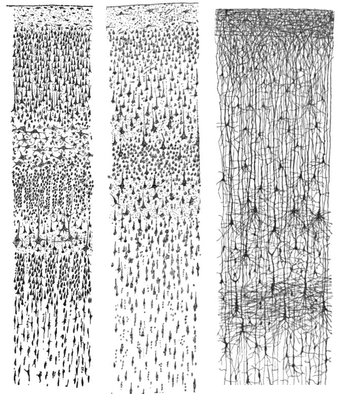
Santiago Ramón y Cajal, three drawings of the layers of the human cerebral cortex
The A-R3 scenarios, why the Neural ODE cannot learn, the DESCARTES-NeuralODE search with an LLM in the loop, eleven architectures that all predict spikes through alien internals, the auxiliary-loss sweep, and the preparations for an L5 pyramidal replication — one hundred and twenty-five questions and their answers
A research guide for the Beniaguev L5PC zombie test, what a report added to it, dendritic voltage traces and loss weights explained, and two visual guides.
A guide mirroring A-R3 on the Hay L5PC model, with up to ~1,800 intermediate variables and a finding in their code: Beniaguev's TCN had a small dendritic-voltage loss.
(Claude looked up Beniaguev's repository and the Hay 2011 model, then wrote the guide as a separate document; it is linked below.)
That's your complete research prompt for the L5PC experiment. The core structure mirrors A-R3 exactly but adapted for a completely different circuit.
The key things to note: Beniaguev's code and dataset are publicly available on GitHub and Kaggle, the Hay 2011 model exposes 12 ion channel types across ~200 compartments giving you potentially 1400-1800 intermediate biological variables (far richer than your 160 thalamic variables), and there's even a minimum viable experiment you can run in one day using their pretrained TCN without re-simulating anything.
The one critical discovery from digging through their training code is that Beniaguev's TCN was actually trained with partial biological supervision — a dendritic voltage trace (DVT) loss component. So you'd want two conditions per architecture: spike-only (your A-R3 paradigm, the pure zombie test) and DVT-supervised (their original setup, which parallels your A-R3b auxiliary bio loss idea). That comparison alone could be a paper.
New: a many-to-one argument that voltage supervision cannot identify gating, a ~20,000× DVT weight ratio, RMMs, Jaxley and the ELM neuron, and an MLP-probe control.
Yes — this document contains several genuinely new pieces that go beyond what we discussed and what's in the guide I made. Let me walk through the important additions.
The theoretical argument for why DVT supervision will fail is now rigorous. We discussed the DVT loss as something to test empirically, but this document lays out five independent theoretical reasons why it cannot propagate to gating variables. The most powerful one is the many-to-one mapping problem: in Hodgkin-Huxley dynamics, different combinations of gating variables can produce identical voltage trajectories (the Prinz/Marder degeneracy). This means even perfect voltage supervision is mathematically insufficient to identify individual gating variables — the mapping is non-invertible. We treated the DVT condition as an open empirical question; this document says the theory already predicts it will fail. That reframes your Condition A vs Condition B comparison from "will it work?" to "confirming the theory predicts it won't work," which is actually a stronger scientific position.
The DVT loss weight quantification is new and devastating. The document calculated that the DVT term contributes gradients approximately 20,000× smaller than spike prediction loss. We noted the loss weights from the code but never computed that ratio. At that magnitude, DVT is essentially a rounding error in the optimization — a "barely-perceptible regularizer" rather than a representation-shaping force. This is a concrete number you can cite.
Three new papers and tools we didn't discuss. First, Burghi et al. (2025, PNAS) introduced Recurrent Mechanistic Models (RMMs) that are hybrid architectures embedding biophysical structure by design — and they successfully recovered HH conductance trajectories. This is the anti-zombie approach: constraining architecture to be mechanistically faithful rather than testing whether unconstrained ones spontaneously are. It's the perfect foil for your work. Second, Mavor-Parker et al. (2024, PLOS Computational Biology) used Multi-gate Mixture-of-Experts to predict all 639 compartment voltages simultaneously — but as output targets, not discovered representations. Third, and potentially game-changing, Jaxley (Deistler et al., 2025, Nature Methods) is a differentiable simulation framework in JAX that enables backpropagation through all biophysical state variables. This could serve as a "gold standard non-zombie comparator" since it's constrained to use biophysical variables by construction.
The ELM neuron recommendation is new and strategically brilliant. Spieler et al. (2023/2024, ICLR) designed the Expressive Leaky Memory neuron with biologically-inspired leaky memory states and showed that Beniaguev's TCN needed ~10M parameters partly due to inductive bias misalignment, while ELM achieves comparable accuracy with only ~8K parameters. The document recommends testing whether ELM's memory states show higher Ridge R² than TCN's hidden states. This directly tests whether biological inductive bias produces less zombie-like surrogates — a finding with immediate implications for prosthetics design. We didn't have ELM in our architecture suite at all.
The nonlinear probing control is an important methodological addition. The document flags that Ridge R² = 0 could mean either genuine zombie (alien representations) OR biological variables encoded nonlinearly. Adding a small MLP probe as a control would distinguish these cases. If the MLP probe also gets R² ≈ 0, it's a true zombie. If the MLP succeeds where Ridge fails, the information is there but in a nonlinearly entangled form — still zombie-like by the linear representation hypothesis, but a weaker form. We didn't include this control in the guide.
Practical NEURON details are more specific. The document confirms the cell variant is L5PCbiophys3, warns that NEURON 9.0 breaks VERBATIM blocks in older mod files (recommending 8.2.6 specifically), notes that synaptic conductances from BlueBrain mechanisms (ProbAMPANMDA_EMS) may need a one-line mod file edit to expose variables via _ref_, and clarifies that the Kaggle dataset does NOT include DVT data despite the paper referencing it during training.
The framing of your work within three disconnected communities is new. The document maps the gap as sitting at the intersection of neural surrogate modelling (who build black boxes), mechanistic interpretability (who probe black boxes but only in language/vision), and biophysical neuroscience (who care about mechanism but never probe surrogates). Nobody in any of these three communities has asked the zombie question. That's a cleaner articulation of novelty than we had before.
Should I update the guide to incorporate these new elements — particularly the ELM architecture, the MLP nonlinear probe control, the Jaxley comparator, and the theoretical impossibility argument for DVT propagation?
Dendritic voltage traces: ~200 compartment voltages compressed to 30 PCA components, a tiny auxiliary loss in Beniaguev's training that cannot pin down gating.
DVT stands for Dendritic Voltage Traces — it's a term specific to the Beniaguev et al. (2021) paper and their training setup.
Here's the idea. The L5 pyramidal neuron has a massive dendritic tree with roughly 200 compartments. During simulation, every single compartment has its own membrane voltage trajectory over time. So at every millisecond, you don't just have the somatic voltage (the "output" at the cell body) — you have 200 voltage traces spread across the basal dendrites, oblique branches, apical trunk, and the tuft. These are the dendritic voltage traces.
Now, storing and training on all 200 raw voltage traces would be expensive and redundant (nearby compartments have correlated voltages). So what Beniaguev did was compress those ~200 dendritic voltage traces down to 30 PCA components — essentially capturing the dominant patterns of voltage variation across the whole tree in a compact form. These 30 compressed traces are what they call the DVT signal.
During training, their TCN loss function had three terms: the main spike prediction loss (weighted at 1.0), a somatic subthreshold voltage loss (weighted at 0.02), and the DVT loss (weighted at roughly 0.000005). That DVT term gently encouraged the network to track what's happening across the dendritic tree, not just predict the somatic output. But as the document points out, that weight is approximately 20,000× smaller than the spike loss — so it's barely nudging the optimization.
The reason DVT matters for your experiment is this: Beniaguev's TCN wasn't trained purely on spike prediction the way your A-R3 architectures were. It had this tiny bit of biological supervision about dendritic states baked in. The theoretical argument in that document is saying that even this supervision is fundamentally insufficient to force the network to learn actual gating variables, because the mapping from gating variables to voltages is many-to-one — different channel configurations can produce identical voltage traces. So supervising on voltages (even dendritic voltages everywhere in the tree) cannot uniquely determine what the individual sodium gates, calcium gates, and potassium gates are doing underneath. The voltage is a summary of all those mechanisms combined, and the combination is not invertible.
That's why your two experimental conditions matter: Condition A (spike-only, no DVT) is the pure zombie test matching your A-R3 paradigm, and Condition B (with DVT supervision, matching Beniaguev's original setup) tests whether even partial biological supervision about dendritic voltages can propagate down to the mechanistic level of individual channel gating variables. The theory says it can't, but proving it empirically is the point.
The loss is a score to shrink; weights say how much each task counts — spikes are the maths exam, dendritic voltages an art grade the network rationally ignores.
Think of it this way.
When you train a neural network, you need to tell it what "doing a good job" means. The loss function is basically a score that measures how badly the network is doing — how far off its predictions are from the correct answers. The network's entire goal during training is to make this score as small as possible. Every time it processes a batch of data, it checks its loss, then adjusts its internal weights to try to reduce it. That's all training is — repeatedly shrinking the loss.
Now, sometimes you want the network to be good at more than one thing simultaneously. Imagine you're training a student and you say: "I care mostly about your math exam score, I care a little about your reading score, and I care just a tiny bit about your art score." You'd combine these into one overall grade, but you wouldn't weight them equally — math counts the most, reading counts some, and art barely matters.
That's exactly what Beniaguev did with three terms in their loss:
Term 1 — Spike prediction (weight = 1.0). This is the "math exam." It measures how well the network predicts when the neuron fires a spike at the soma. This is the main job, so it gets the highest weight. If the network gets spikes wrong, the loss shoots up and the network gets heavily punished.
Term 2 — Somatic subthreshold voltage (weight = 0.02). This is the "reading score." Between spikes, the membrane voltage at the soma wobbles up and down without reaching threshold. This term checks whether the network predicts those subthreshold wiggles correctly. It's weighted at 0.02, meaning it matters about 50× less than spike prediction. It's helpful but secondary.
Term 3 — DVT / dendritic voltages (weight ≈ 0.000005). This is the "art score." Those 30 PCA-compressed voltage traces from across the dendritic tree? The network gets a tiny reward for tracking them correctly. But the weight is so absurdly small — about 200,000× less than spike prediction — that it barely influences what the network learns. It's like telling the student "oh, and your art grade counts for 0.0005% of your final mark." The student will rationally ignore art and focus entirely on math.
The weight on each term determines how much the network cares about that particular task during training. When the network computes its gradients (the direction to adjust its internal parameters), each loss term contributes a gradient proportional to its weight. A term with weight 0.000005 produces gradients 200,000× smaller than a term with weight 1.0. Those tiny gradients get drowned out by the spike prediction gradients, so the network's internal representations are shaped almost entirely by what's needed to predict spikes correctly. The dendritic voltage information is, practically speaking, invisible to the optimizer.
This is why the theoretical argument says DVT supervision "will fail" at forcing biological correspondence. Even though the network is technically being told "try to track dendritic voltages too," the instruction is whispered so quietly compared to the spike prediction instruction that the network essentially ignores it. And even if you turned the DVT weight way up, there's a deeper problem — knowing voltages doesn't uniquely tell you what the individual ion channels are doing underneath, because many different channel combinations can produce the same voltage. So even loud voltage supervision can't force the network to learn individual gating variable dynamics.
Nine animated chapters from the neuron to the DESCARTES framework, with dental analogies.
(The guide was built as a separate interactive file; it is linked below.)
Here's your interactive visual guide with 9 chapters that build from the absolute basics up to your DESCARTES framework. Each chapter includes animated diagrams, dental analogies you can relate to, and highlighted key insights. Navigate through chapters using the tabs at the top or the Previous/Next buttons at the bottom.
The chapters flow as: Neuron → Ion Channels → Action Potential → Gating Variables → Compartmental Models → Neural Network Surrogates → The Zombie Problem → The Zombie Test (Ridge R²) → DESCARTES & Your Work. By the time you've read through all nine, the technical guides should make much more sense — every term like "gating variable," "compartment voltage," "Ridge R² = 0," and "DVT loss" connects back to concrete visual concepts in this guide.
Ten sections from HH equations and the loss function to the Pearson trap and philosophical implications, all with the actual numbers from the runs.
(The first reply was cut off; after “Continue”, Claude built the guide as a separate interactive file, linked below.)
Here's your advanced Le Masson guide with 10 sections covering the full mathematical and philosophical depth of the A-R3 experiment. Hover over circuit components for contextual tooltips.
The 10 sections are: Circuit Biology (HH equations, bifurcation threshold, I_T gating), Ground Truth Data (190 trials, 160 variables breakdown), Loss Function (BCE + MSE with gradient analysis and weight philosophy), Progressive Curriculum (4-stage dynamics and LR trap), 11 Architectures (full results table with ODE/LTC/GRU-ODE/hierarchical dynamics), Training Dynamics (speed tiers, val loss convergence ceiling), Zombie Test (Ridge R² math with 5-fold CV), Pearson Trap (the r=0.98 mirage vs R²=0.0001 reality), Complete Results (scatter plot showing all points at zombie floor), and Philosophical Implications (functionalism, biological naturalism, gradual replacement consequences).
Every section includes the actual equations, real numbers from your runs, and connects back to the substrate independence question.
Files written in the conversation and research reports uploaded into it. Files Claude wrote are hosted in the reports/ folder beside this page; report filenames are descriptive placeholders for the files Charith uploaded, which are not yet hosted.
The questions are Charith’s, corrected for grammar and spelling only. The answers are Claude’s, as given in the conversation; tool calls, file contents and research prompts are omitted and noted where they occurred. The model label is inferred from the date of the conversation.
Source: claude.ai project “La Masson 2002”, conversation of 24 February 2026, “Neural ODE evaluation incomplete, Volterra and LSTM latent structure results”.